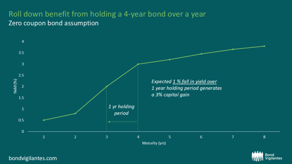
Rolldown
A dispatch from the number crunchers – Yield curve rolldown
By Matthew Russell
15 April 2026

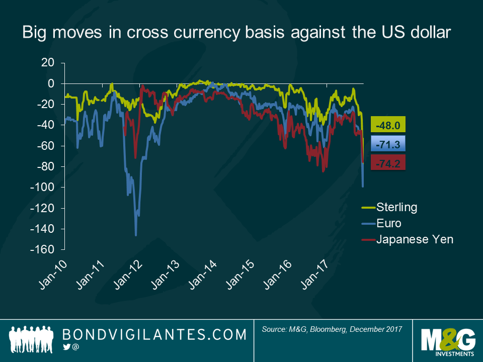
Towards the end of this year, a December spike in the cross currency basis for major currencies against the dollar grabbed the market’s attention. But what is cross currency basis (“the basis”)?
Consider a European company taking a one year loan from its domestic local bank to fund its US operations abroad. In order to hedge the currency risk, the company enters into a one year EUR/USD currency swap with a market counterparty. The European company swaps a certain amount of Euros for US Dollars at today’s spot rate, agreeing to swap the funds back at the same rate in one year’s time. Because the European company doesn’t technically own the US Dollars, it will need to pay back US Libor as interest and by reciprocity, receive Euribor from its counterpart. This is how it should work in theory (i.e. according to covered interest rate parity).
In practice, however, whenever there’s a higher demand for the dollar, the counterparty lending the dollar will ask for a price premium. It is this amount which is referred to as the “cross currency basis”. In other words, the European company will pay out US Libor and will receive Euribor plus the cross currency basis (quoted as a negative figure).
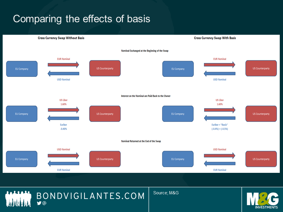
Let’s look at an example: If today US Libor is 1.6% and Euribor is -0.4%, the theoretical cost of the EUR/USD currency swap to the European company is 2% (i.e. it pays out 1.6% on the dollar interest, but also pays out 0.4% on the Euro interest because Euribor today is negative). If, due to a dollar shortage, the counterparty quotes a “basis” of -50 bps, then the cost of this swap to the European company would increase to 2.5% (1.6% Dollar interest + 0.4% Euro interest + 0.5% currency basis).
In general, the cross currency basis is a measure of dollar shortage in the market. The more negative the basis becomes, the more severe the shortage. For dollar-funded investors, negative basis can work in their favour when they hedge currency exposures. In order to hedge foreign currency exposure, the dollar-funded investors lend out dollar today and receive it back in the future, earning additional cross currency basis spread on top of the yield of their foreign investments. In fact, for years the Reserve Bank of Australia has been swapping its other foreign currency reserves against the Japanese Yen in order to enhance returns. After taking the basis into account, negative yielding short-term Japanese government bonds actually yield higher than many short-term government bonds in other currencies.
For foreign investors, however, the basis could increase their hedging cost of investing in the dollar assets. In order to hedge dollar exposure, foreign investors borrow dollar today and return it back in the future. The basis is the additional hedging cost added to the interest differential of the two currencies.
Cross currency basis is an important part of currency management in a global portfolio. Given that the Fed is now well ahead of the ECB and other central banks in its monetary tightening cycle, it is likely that the dollar shortage could heighten in the coming year, and the basis could become more negative. Portfolio managers should be mindful of the hedging cost when taking foreign currency positions.
Short term US dollar interest rates continue their march higher. 3-Month USD LIBOR recently hit 1.61%, fuelled by the Fed’s 25 basis point hike on December 13th, a level last seen in late 2008. With further rate hikes on the horizon in the US and a potentially more hawkish European Central Bank, is 2018 the year when floating rate high yield meaningfully outperforms its fixed rate cousin?
The short answer is: “probably yes” for a EUR investor and a somewhat unsatisfying “maybe” for a USD investor.
Looking at a simple scenario analysis for 1 year total returns, I take two theoretical USD portfolios (one of high yield floating rate notes and the other high yield fixed rate bonds), both priced with a spread of 250bps to normalise the relative impact to returns, and flex the total return of each portfolio to take into account three rate hikes from the Fed (the current market consensus view) and a change in yield curve (i.e. a move that would mean an interest rate duration related capital gain or loss for the fixed rate portfolio).
It should be noted, however, that I have not considered the relative impact of a move in credit spreads or default rates, which is another very important driver of returns for high yield. I would expect floating rate high yield to outperform fixed rate high yield in a spread-widening sell-off or if we saw higher default rates (floating rate bonds tend to have less spread duration and are more heavily skewed to senior secured instruments), and vice versa. The numbers below do not take this into account.
The results above show that the market would need to see a moderate move higher in US treasury yields before floating rate high yield outperforms fixed rate high yield. In fact, the breakeven level is 34bps in this case. Some hikes are already reflected in the steepness of the US treasury curve at the front end, so investors are already to some extent compensated for the fact that the Fed is maintaining its hawkish stance. Floating rate high yield would be better placed to outperform if we saw more than three hikes or if a subsequently more hawkish stance was priced into the fixed rate market. The perception that floating rate bonds outperform when interest rates are rising in not always true.
| USD – (three hikes and steeper/flatter yield curve)
|
||||||||
| Change in yield (bps) | -75 | -50 | -25 | 0 | 25 | 50 | 75 | |
| FRN HY 1yr total return | 4.42% | 4.42% | 4.42% | 4.42% | 4.42% | 4.42% | 4.42% | |
| Fixed HY 1yr total return | 8.73% | 7.75% | 6.76% | 5.77% | 4.78% | 3.80% | 2.81% | |
How about EUR based investors? Below is the same exercise, but I assume no change to EURIBOR at -0.39% (i.e. no hikes from the ECB), but flex the yield curve as before.
| EUR – (no hikes and steeper/flatter yield curve)
|
|||||||
| Change in Yield (bps) | -75 | -50 | -25 | 0 | 25 | 50 | 75 |
| FRN HY | 2.11% | 2.11% | 2.11% | 2.11% | 2.11% | 2.11% | 2.11% |
| Fixed HY | 5.29% | 4.33% | 3.38% | 2.42% | 1.47% | 0.51% | -0.45% |
What is interesting here is that the flat government bond curve works against fixed rate investors. European government bond yields would have to sell off by only 8bps before floating rate high yield outperforms. Any marginal repricing of ECB intentions to a more hawkish scenario, therefore, would mean investors are much better off in floating rate bonds, not because they benefit from higher coupons as interest rates rise, but rather because they have almost zero sensitivity to moves in the government bond markets.
It’s Christmas jumper time! In our final BVTV of 2017, fund manager Ben Lord joined me to assess bond market returns this year and share his thoughts on the outlook for growth and UK monetary policy.
Tune in to hear Ben’s credit views, and what’s on his wish-list for markets in 2018.
Here’s a short video I recorded with my multi-asset colleagues Steven Andrew and Tristan Hanson, in which we debate the highlights of 2017 and look ahead to 2018. After a year that has turned out to hold fewer surprises than many might have expected, what lies in store for financial markets in the coming 12 months?
Yesterday we saw Inter Milan issue the first football related high yield bond since we saw Manchester United tap the market back in January 2010. Putting aside the natural tribalism of 2 of my esteemed colleagues (both Italian, both ardent AC Milan supporters), we decided not to invest in the €300m 4.875% 2022 bond.
In terms of fundamentals, legal claim, and relative value, the bond stacks up fairly well. Inter Milan is a well-established club with a solid fan base and is currently top of the table in Serie A. As such the club is well placed to generated sustainable revenue from broadcast rights and monetise its brand through sponsorship deals. The risk to revenue, at this stage at least, from sustained poor performance on the pitch seems low. This is important as the bond is structured in a way that means bondholders are effectively lending against the cash flow generated by the club’s media and sponsorship agreements, not the cash flow of the club as a whole. Crucially, this removes a major potential negative factor: the issue of cost inflation in the form of ever-increasing wage demands from players.
Also, at 4.875% for a BB- rated bond, the coupon looks good value compared to the rest of the European High yield market with average yields for BB corporates at 1.8% and 2.5% for the high yield market as a whole.
So what’s the problem? In our view the key issue is how the bond’s maturity profile and potential cash flow is mismatched. The bonds are subject to the following amortisation schedule:
Mandatory Amortization Redemption and Principal Repayment Date Principal Amount
December 31, 2018 . . . . . . . . . . . . . . . . . . . . . . . . . . . . . . . . . . . . . . . . . . . . . . . . . . . € 3,100,000
June 30, 2019 . . . . . . . . . . . . . . . . . . . . . . . . . . . . . . . . . . . . . . . . . . . . . . . . . . . . . . . € 3,150,000
December 31, 2019 . . . . . . . . . . . . . . . . . . . . . . . . . . . . . . . . . . . . . . . . . . . . . . . . . . . € 3,250,000
June 30, 2020 . . . . . . . . . . . . . . . . . . . . . . . . . . . . . . . . . . . . . . . . . . . . . . . . . . . . . . . € 3,300,000
December 31, 2020 . . . . . . . . . . . . . . . . . . . . . . . . . . . . . . . . . . . . . . . . . . . . . . . . . . . € 3,400,000
June 30, 2021 . . . . . . . . . . . . . . . . . . . . . . . . . . . . . . . . . . . . . . . . . . . . . . . . . . . . . . . . € 3,500,000
December 31, 2021 . . . . . . . . . . . . . . . . . . . . . . . . . . . . . . . . . . . . . . . . . . . . . . . . . . . . € 3,550,000
June 30, 2022 . . . . . . . . . . . . . . . . . . . . . . . . . . . . . . . . . . . . . . . . . . . . . . . . . . . . . . . . € 3,650,000
December 31, 2022 . . . . . . . . . . . . . . . . . . . . . . . . . . . . . . . . . . . . . . . . . . . . . . . . . . . €273,100,000
In this case, the amortisation is welcome, but the amounts that are mandatorily repayable seem insignificant relative to the outstanding amount of debt. Over €270m of an original €300m issued is effectively a bullet maturity. At the same time, if the club meets certain financial tests, any surplus cash flow generated by broadcast and media rights can then be distributed to other entities over which the bondholders have no legal recourse. This could mean, in extremis, that the structure re-leverages over the life of the bond with increased re-financing and credit risk even if the club performs well and monetises this success.
So despite being undisputedly the best football club in Milan right now, we think the devil is in the detail when it comes to Inter’s debut bond issue.
In our latest Panoramic Outlook, Jim Leaviss assesses the forces behind the robust and broad-based nature of global economic growth in recent months and the prospects for this broadly rosy outlook continuing into 2018. He looks at where we are within the current global deleveraging cycle, and asks how high this means that rates can go. In Jim’s view, the quality of investment grade credit has seen significant deterioration in recent years, another factor that is particularly important when considering whether credit spreads can compress further as we go into 2018.
For this and more, please view our 2018 outlook.
Here is the 11th annual Christmas Quiz. 20 questions, and the closing date for entries is midday on Friday 22nd December. Please email your answers to us at bondteam@bondvigilantes.co.uk. The winner will get glory, and in lieu of a golden trophy, M&G has donated £500 to Cancer Research UK, through CASCAID. CASCAID is the UK asset management industry’s effort to raise £2 million for this brilliant charity over the course of 2017.
Breaking news: we did it! But please help us raise a few final pounds by the end of the year. If you’d like to donate a fiver as you enter, please do so at my charity page here https://uk.virginmoneygiving.com/fundraiser-display/showROFundraiserPage?userUrl=JimLeaviss&pageUrl=2 but it is totally optional, and I know a) many of you have been incredibly generous already, and b) I have bored on about cycling up hills enough for one year.
Good luck! Conditions of entry of down below somewhere.


Good luck!
Richard recently wrote about how government bond indices should be adjusted to account for quantitative easing (QE) purchases, thereby better reflecting the actual availability of investments in the market. A key argument indicated that given the absence of this adjustment, European government indices are incorrectly skewed towards more highly rated sovereigns, even though their issuance is not freely available to purchase.
I have expanded on this work to assess this idea on a global scale using the ICE Bank of America Merrill Lynch Global Government Bond index (i.e. reweighting the index to adjust for the QE undertaken in Europe, the US, UK and Japan). Though the premise remains the same – i.e. that bond indices should look different in a QE adjusted world – the impact at the global level differs from the European analysis in two key ways.
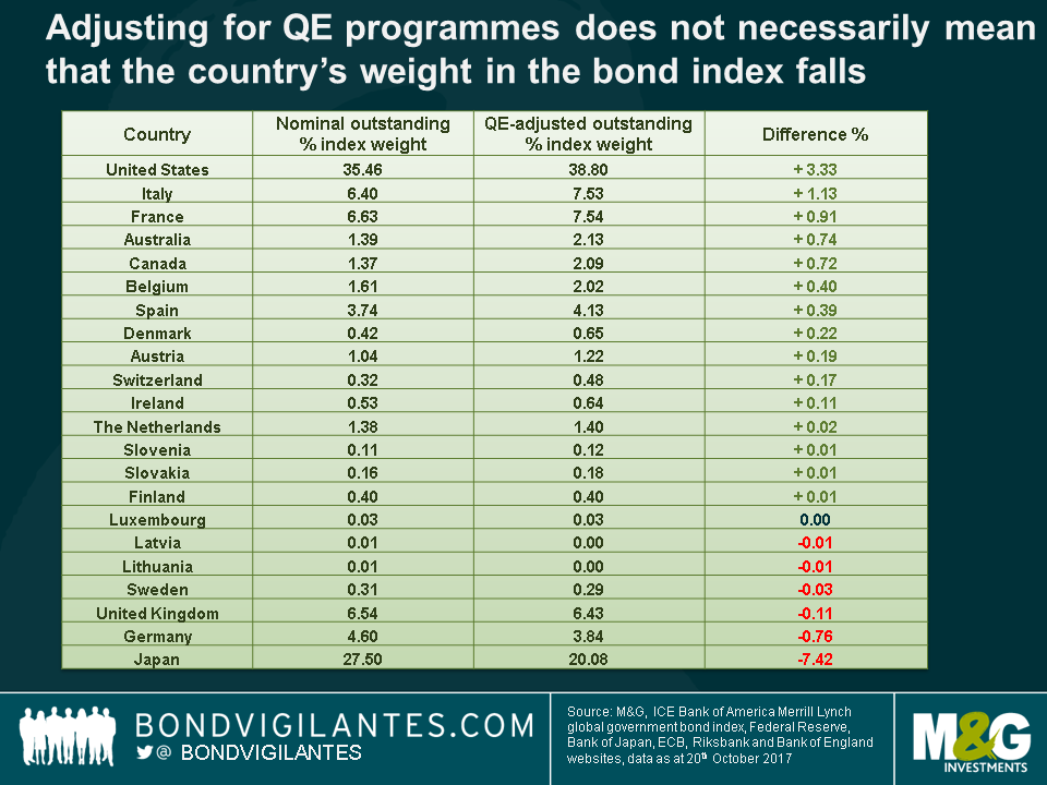
Broadly speaking, I had anticipated that countries which had undergone QE would see their weights in the index reduced, while other country weights (i.e. those which did not do QE) would rise. Looking at the table below, though this was indeed the case for countries where central banks continue to undertake wide-scale QE (e.g. Japan, Germany, Sweden) or where this has been conducted previously (e.g. in the UK, most recently after the EU referendum), I did not expect the change at the top of the table where the US has increased its weight by 3.33%.
Though the US has itself completed $2.5tn worth of government bond QE, this is dwarfed by the ¥400tn (approx. $3.5tn as at 20th October) worth of ongoing QE conducted by the Bank of Japan. Adjusting the index for the free-float of government bonds, Japan – the second largest weight in the index, but the country with the largest QE program – sees its available investment universe fall considerably and hence its index share is reduced from 27% to 20%. On the other hand, though the US investment universe has also decreased, its outstanding issuance remains large. As a result, the US manages to retain its proportional top spot in the index, increasing its weight from 36% to 39%.
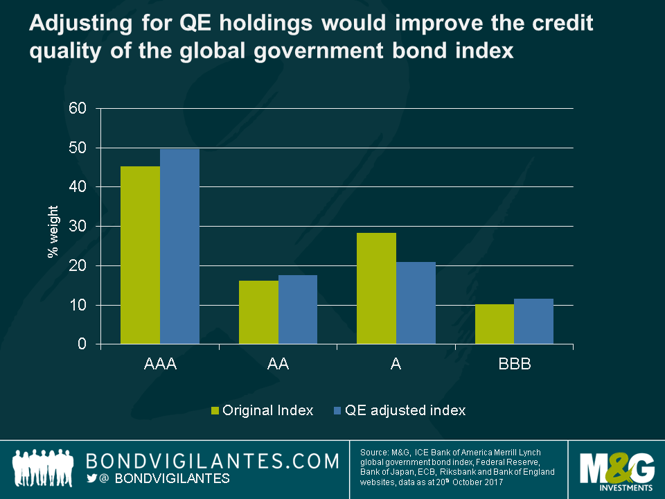
In the previous European focused blog, we showed that adjusting for QE causes higher rated countries like Germany to lose weighting in the index to lower rated countries such as Italy and France. This trend does persist at the global level, but the aforementioned reduction in Japanese holdings has a secondary meaningful impact. Since Japanese government bonds are rated A, the reweighting away from this country towards others such as the US, Australia, Canada which are more highly rated, means that the overall index actually improves in credit quality (67% rated AAA or AA, compared to 62% previously). This is in contrast to the European index where the credit quality deteriorates.
This analysis has interesting practical implications. We argued previously that tracker funds, following European indices that are not QE adjusted, are potentially driving up European government bond prices (i.e. being forced buyers in an environment with reduced free-floats). Although the same case could be made for Japanese government bonds, US Treasuries are arguably under bought.
This week Stefan Isaacs joins me to review the year that was. Sitting on a bond desk in the City of London, it appeared to be a solid but pretty dull year for fixed income markets. Fortunately, we had the drama of Brexit negotiations and Donald Trump to keep us occupied over the course of the year.
I also question Stefan about his 2018 outlook for bond markets, and whether Liverpool can actually go all the way and win the UEFA Champions League. Spoiler alert: no.
After four calendar years of price appreciation, it looks like the US dollar will end 2017 deeply in negative territory. The dollar has fallen by almost 12% this year versus the euro and around 8% on a trade weighted basis. More surprisingly, the sharp depreciation of the dollar against the euro has occurred in a period when central bank policy has diverged, resulting in the yield differential between 2 year US Treasuries and German Bunds widening, going against the broad relationship of the past 10 years.
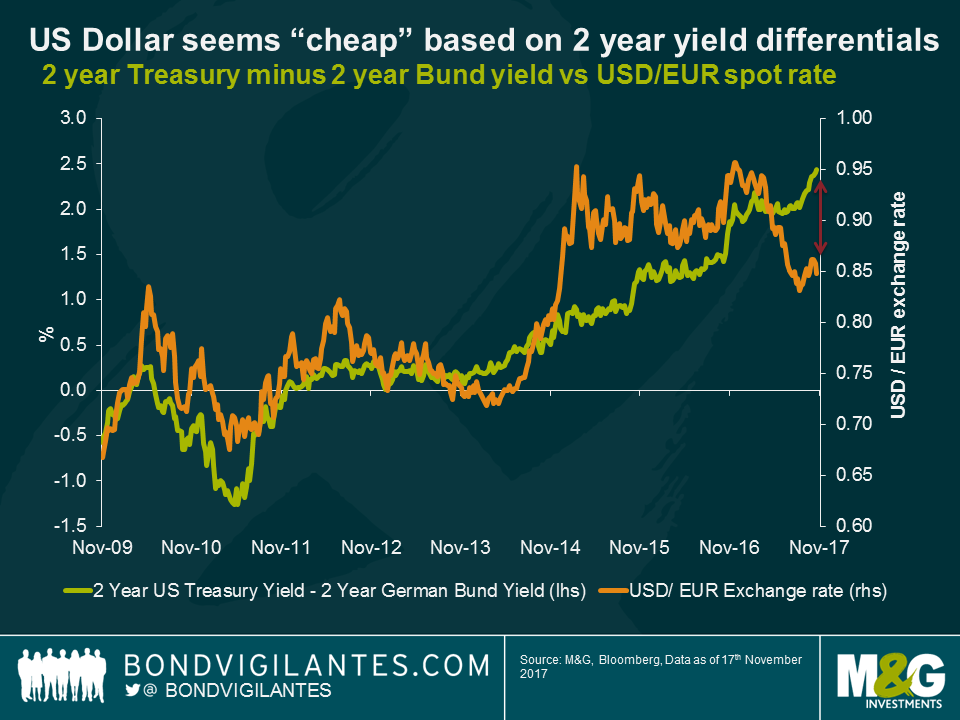
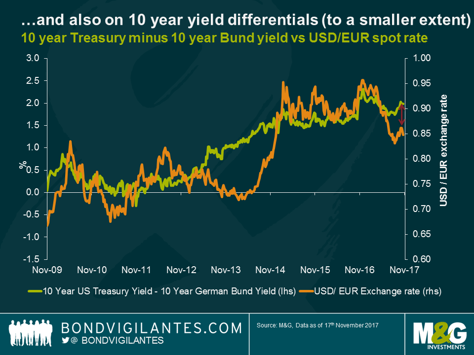
We recently pointed out some some of the reasons behind the US dollar’s weakness versus the euro despite rising yield differentials here. In addition, it’s worth pointing out that the current dislocation between US and European government bond yields and currencies is probably exacerbated by two additional and slightly more technical factors. Firstly, given the fact that the ECB has been buying a disproportionate amount of Bunds relative to other European government bonds, the current Bund yield is significantly depressed, increasing the yield differential with US Treasuries. If the US versus Europe yield differential is calculated using a capital key weighted average of German, French, Dutch, Belgium, Spanish, Italian, Portuguese and Irish 2 year government bonds instead of Bunds, the EUR / USD dislocation does not appear as extreme. Calculated in this way, 2 year European yields would be approximately 0.2% higher, reducing the yield differential with Treasuries by around the same amount. Secondly, the flat shape of the US yield curve suggests the US dollar is not as cheap relative to the euro as the 2 year differential chart would suggest. If 10 year US Treasury versus German Bund yield differentials are used, the US dollar still looks undervalued, but to a smaller extent.
Nonetheless, even using the slightly modified methodologies mentioned above, the USD still appears undervalued versus the Euro relative to what the yield differential would suggest. Given that this relationship has been quite strong since the global financial crisis, an interesting exercise has been to look at the relationship from a longer term perspective in order to compare the current valuation gap to what has occurred historically. By chain linking movements of the underlying euro currencies to the euro before 1999 and comparing them to the difference between 2 year Bund yields and 2 year Treasury yields, I produced the chart below, which goes back to the mid 1970’s.
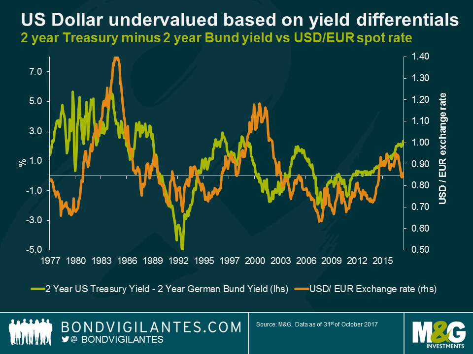
While taking a longer term view confirms that there is a positive relationship between yield differentials and the USD/EUR exchange rate, it also shows that over the past 40 years there have been times when the relationship has broken down quite drastically. One of the reasons this may be the case is that in the 70’s and 80’s, capital markets were not as global as they are today, so investors were less able to arbitrage yield differentials between the US and Europe (i.e. Germany before 1999 in this case) in the same way.
In addition, the fact that bond yields have fallen quite dramatically over the period makes interpreting the chart more challenging, as one is less likely to see today the same level of yield divergence as in the past. One way to adjust at least in part for this factor is to use real yield differences (which I have approximated in the chart below by using nominal yields minus trailing year-on-year inflation rates) rather than nominal yields and compare these to the historical USD/EUR exchange rate.

The chart above shows that adjusting for differences in inflation between the US and Germany improves the relationship significantly, especially during times of inflation surprises or significant inflation divergences between the two countries. Another argument that can therefore be put forward to explain the USD “cheapness” today when measured by yield differentials is that it may have been caused by consistently higher inflation expectations in the US relative to Europe in recent times.
Over the past forty years there have been a couple of instances where the relationship between yields and exchange rates have broken down for a prolonged period of time. The first of these two instances occurred between Q1 1994 and Q1 1996 and coincided with what is known as “the Bond Massacre” (we have previously written about this here), a period where the US Fed hiked rates by 2.5% in a single year, wreaking havoc in bond markets. The second instance was from early 1999 to late 2002 and corresponds to a major confidence crisis for the newly introduced euro (the euro had a rough start, see here for example).
Despite the relationship breaking down more recently, the yield differential between two year US Treasuries and 2 year German Bunds remains a relatively good predictor of exchange rate movements over the long term. Those predicting further weakness of the US dollar relative to the euro in 2018 (the forwards market suggests EUR/USD at 1.21 in Q4 2018 despite expectations of further rate hikes from the Fed) would do well to remember this relationship.


Sign up to the Bond Vigilantes mailing list to ensure you never miss a great article from our expert Bloggers. We will email all new articles to your inbox, meaning you can stay on top of the world of Bonds.
I confirm that I would like to receive information about Bond Vigilantes and products and services from M&G Securities Limited.
We will use the email address and personal data you have shared with us to send you this information. For existing customers, submitting your contact details and requesting to receive this information from us, will replace any earlier choices you have made in respect of marketing information.
You can unsubscribe from marketing at any time, at which point we will not send any further marketing information to you, by selecting the unsubscribe link in all communications.